Biotracing for Experts
This part of the web-site describes the details of the Operational Biotracing system deployed under this web-site. The example is taken from [1].
In the following sections describe the Bayesian network modules that represent uncertain beliefs concerning the coupled dynamics of Staphylococcus aureus, staphylococcal enterotoxins and alkaline phosphatase in the small scale processed milk chain.
The complete Bayesian network Risk Assessment Model for Enterotoxigenic Staphylococcus aureus in Pasterurized Milk is shown in Figure 1.
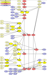
Figure 1: The milk model.
It enables a potential route to source-level inference. To interact with the model scroll down.
Milk Pooling
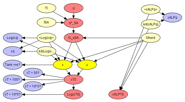
Figure 2: The milk pooling module.
On the farm milk is collected from individual dairy cows and pooled in a single holding tank. Individual animals can contribute S. aureus, and alkaline phosphatase (ALP), at different rates so that the pooled volume has a complex distribution of potential bacterial and enzymatic loads. These distributions can be constructed from distributions for individual quarter components and from an assumption that the properties of milk from different bovine quarters within a herd are independent. In the network representation the number of quarters that contribute contaminated milk (N_qSA) and the quarter concentration of ALP (cALPq) are dominant input variables and the logarithm of the tank concentration of S. aureus (Log(CT0)) and the tank concentration of ALP (cALPT0) are dominant output variables. The number of animals in the herd (Nherd) is a dominant source of variability in the output values.
Cooling Tank Milk
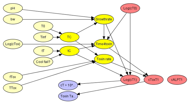
Figure 3: The cooling tank milk module.
Rapid cooling, following milk collection, is an important element of food safety. The cooling is usually under strong control and reduces milk temperatures to ~4-6C over a period of about 2 hours. The temperature history, over the cooling period, determines the ultimate quality of farm tank milk. The model includes a possibility for unobserved failure in the cooling process and a logical variable CoolFail? In the event of failure the time of cooling (tC) is extended and the mean temperature during the cooling (TC) is elevated. The two variables representing the cooling process can be combined with a predictive microbiological model to estimate belief concerning the logarithm of the concentration of S. aureus (Log(cT1)) and the concentration of staphylococcal enterotoxin (cToxT1) that exist in the farm tank after the cooling process. Additional uncertain parameters, such as water activity (bw) and the toxigenic fraction of S. aureus (fTox), are included in the development of beliefs concerning the development of contamination. The cooling process does not have any effect on the concentration of ALP in milk so that the variable representing tank concentration (cALPT1) is disconnected from other variables in the module. Changes in belief concerning cooling failure have strong effects on the S. aureus concentration and the enterotoxin concentration in cooled tank milk. Changes in belief about physicochemical parameters of milk are less significant.
Milk Pasteurization
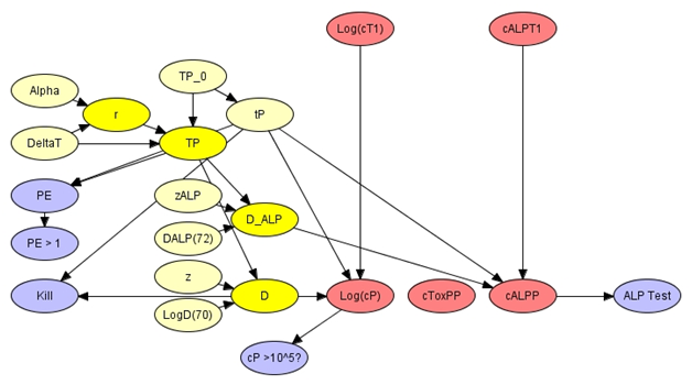
Figure 4: The milk pasteurization module.
A pasteurization step is central to the processing of milk for human consumption. During pasteurization milk is heated to a target temperature (TP_0) for a fixed period (tP) to eliminate important pathogens. In a few cases, representing failures, the process might be incomplete so that the milk is heated at a lower temperature (TP). Linear models can be used to predict the changes in concentrations, for S. aureus (Log(cP)) and ALP (cALPP), that result from thermal processing. Uncertainty surrounding the thermal inactivation of bacteria and enzymes in included in parameters (LogD(70), z etc.) of the model. The efficiency of the pasteurization can be represented by a logical variable (PE > 1) that compares the actual process to an established standard (which is usually heating at 72C for 15s). This variable also acts as an indicator of beliefs concerning unobserved pasteurization failures. The module can also, productively, include a Boolean variable (ALP Test) that expresses belief concerning the result of a standard test for ALP. Pasteurization has no effect on staphylococcal enterotoxins, which are heat stable, so that the post pasteurization concentration of toxin (cToxPP) does not depend on pasteurization properties and is disconnected from other variables in the module.
Contamination of Processied Milk
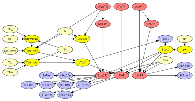
Figure 5: The contamination of processed milk module.
Following processing there are additional opportunities for milk to become contaminated with S. aureus and with enterotoxin. Most notably these processes correspond with the re-introduction of small amounts of unprocessed milk into the supply as a result of faulty operations in separation, packaging etc. The contamination module expresses beliefs about the logarithm of the concentration of S. aureus (Log(cF)), the concentration of enterotoxin (cToxF) and the concentration of ALP (cALPF) in filler tank milk based on a homogeneous mixing of pasteurized milk with a small amount of unprocessed milk. The unprocessed milk may have been subject to a period when bacterial growth and toxin production were possible so the contamination includes elements of predictive microbiology that match those in the cooling module. Since the contamination module includes a mixing process both the farm tank variables (e.g. Log(cT1)) and post pasteurization variables (e.g. Log(cP)) are included explicitly. The contamination module includes variables that quantify the uncertainties associated with post process contamination, such as the volume fraction of contaminating milk (PhiX) and the effective temperature of contaminated milk (TX) etc., and a Boolean variable (BoolX?) which expresses beliefs about the frequency of unobserved contamination events. The filler tank is the location of many end point observations, such as microbiological assays and ALP tests, and the contamination modele includes corresponding indicator variables.
Network Construction
The four network modules provide the building blocks for a Bayesian network that models the development of contamination, and enzymatic marker concentrations, in the processed milk chain. Modules can be used individually or combined into a single tool for risk assessment. The explicit inclusion of failure variables (CoolFail?, PE > 1 and BoolX) also means that output observations can be used to make inferences about potential sources of failure and hence about the likely sources of S. aureus hazards.
Likelihood Ratios
Bayesian networks evaluate and display posterior probabilities based on the propagation of observations or evidence within a consistent framework of beliefs. Often the posterior probabilities are very informative and help with understanding of evidence and with decision making. However in some scenarios, and particularly in legal frameworks, output probabilities are converted to likelihood ratios to assist with decision making. A likelihood ratio expresses the value of the evidence in leading to a particular conclusion and, to some extent, reduces the dependency of the results on particular probability assignments during modelling. Likelihood ratios are particularly easy to compare (linearly comparable) so this transformation makes complex information easier to interpret. Ultimately biotracing provides support for decision making, e.g. where to initiate remedial actions or whether to search for a hidden source of contamination in a food chain system, and likelihood ratios are the best way to account for these choices.
Operational Biotracing
Although statistical analyses and inference schemes are central to biotracing it is equally clear that in real situations biotracing will involve many other contributory activities. Information systems, surveillance systems, alert systems and decision making systems are all part of a practical food chain biotracing system. Recent developments in molecular markers, in rapid methods and in computer technology make many of these elements practical and timely. Operational biotracing could lead to improved efficiency, improved opportunity for development and improved confidence in controls as well as improved food safety. Biotracing suggests that systematic surveillance and analyses can soon become superior to precedent and subjective judgments in decisions concerning the sources of food borne hazards.
Evidence Variables
Listed below are the possible evidence variables. Variables are grouped according to the possible observations. The evidence concerns filler tank observations for ALP concentration, S. aureus concentration and SE concentration.
| S. aureus Concentration (cfu/mL) | Observation |
| 10^2 < cf | |
| 10^3 < cf | |
| 10^4 < cf | |
| 10^5 < cf |
| ALP Concentration (mU/L) | Observation |
| Select concentration level |
| SE concentration | Observation |
| 0 < cToxF | |
| 0.2 < cToxF |
| Herd size |
Likelihood Ratio Values
The Likelihood Ratio Values p(e|S) / p(e|not S) summarizing source-level inference for the Model describing On-Farm Processing of Milk are computed below. The user should select the appropriate observations above. The probability of each source is shown below the likelihood ratios.
| CoolFail | PE < 1 | BoolX |
| P(CoolFail) | P(PE < 1) | P(BoolX) |
Compute Likelihood Ratios
Press the Compute LRs button below to complete the above table with Likelihood Ratios for the three sources listed in the table
Press the Initialize Reset button to remove entered and computed values and initialise the underlying network
Scenarios
Using the drop-down menu below the user can select input values corresponding to a set of predefined scenarios. The aim is to simplify the process of entering data and to support efficient analysis. This may support, for instance, what-if analysis.
The values corresponding to a predefined scenario may be changed or adjusted by the user.
Select a predefined scenario for easy analysis
Loading Data and Saving Data
The user has three options to upload data from local disk and download data to local disk.
- The first option is to download the data entered in the forms above to a HUGIN case file on local disk. This makes it, for instance, possible for the user to store entered information for easy access at a later point in time, for further analysis in another application (i.e., HUGIN Graphical User Interface), or for record keeping.
- The second option is to upload a case from a HUGIN case file file on local disk. This option can, for instance, be used to load the HUGIN case file stored on local disk using the first option.
- The third option is to upload a set of cases from a HUGIN data file on local disk. A HUGIN data file usually contains a set of cases (as opposed to a HUGIN case file, which only contains a single case). The data cases in the HUGIN data file will be uploaded to the server be processes sequentially. For each case in the data file, the corresponding data is entered into the HUGIN model and a belief update is performed. The results of the belief updates are shown as a table in a separate window (the user may have to allow pop-up windows from this site in order to be able to see the results).
Download to local disk
Download current case (to store entered information on local disk):
The file will be stored using the format of HUGIN case files.
Upload from local disk
Load a case file from local disk: The uploaded file should adhere to the format of HUGIN case files.
Upload a batch of cases from local disk to be processed
Load a case file from local disk: The uploaded file should adhere to the format of HUGIN data files. This is an example file.